An Empirical Study of Training Stability in Feedforward Neural Networks
Abstract
Weight initialization plays a critical role in neural network optimization by influencing early gradient flow, convergence speed, and training stability. While theoretically motivated initialization schemes such as Glorot (Xavier) and He (Kaiming) are widely adopted, their practical behavior depends on architectural and optimization context. This study isolates the effect of weight initialization in a controlled feedforward network trained on a two-dimensional nonlinear classification task. Using a fixed architecture, optimizer (Adam, learning rate 0.001), and dataset split, we compare small normal initialization (std = 0.01), Glorot normal, and He normal across multiple random seeds. Results show that initialization significantly impacts convergence dynamics and run-to-run variability, even when final accuracy is similar. Glorot normal initialization demonstrated the most stable and consistent behavior under these conditions. Qualitative visualization of weight evolution further supports observed differences in optimization stability. These findings highlight that initialization remains a first-order design choice, influencing not only training stability but also time-to-convergence and computational cost.
1. Introduction
Training stability and convergence speed in neural networks are influenced by a combination of architectural choices, optimization strategies, and initialization schemes [1, 2]. Among these factors, weight initialization plays a foundational role by determining the scale and distribution of signals propagated through the network at the start of training. Poor initialization can lead to vanishing or exploding activations and gradients, slow convergence, or highly variable training outcomes across runs [3, 4].
Over time, several theoretically motivated initialization strategies have been proposed to address these issues. Glorot (Xavier) initialization was introduced to preserve signal variance across layers in networks with saturating nonlinearities such as sigmoid and tanh [4]. He (Kaiming) initialization was later derived to better accommodate rectified linear units (ReLU) by explicitly accounting for the asymmetric activation behavior of rectifiers [5]. These methods are now widely adopted as default initialization schemes in modern deep learning frameworks.
Despite this theoretical grounding, the practical effectiveness of an initialization strategy depends on more than the activation function alone. Factors such as input dimensionality, layer width, network depth, optimizer dynamics, and learning rate selection all influence how initial weight distributions translate into early training behavior [2, 6]. In practice, initialization is often treated as a secondary concern (particularly when normalization layers or adaptive optimizers are employed) which can obscure the role initialization plays in shaping optimization dynamics, especially in smaller or simpler models. The objective of this study is to isolate and empirically evaluate the impact of weight initialization on training behavior under controlled conditions. Using a fixed dataset, architecture, optimizer, and learning rate, we compare three initialization strategies:
- Small normal
- Glorot normal
- He normal
Each configuration is evaluated across multiple random seeds to assess convergence speed and run-to-run stability. Normalization layers are intentionally omitted to expose initialization effects directly.
1.1 Implementation Artifacts
This study uses a company developed neural network framework (SaorsaNN_CPU.py). The experimental workflow is organized into four core components:
- Dataset generation and train/validation splitting: Held constant across all runs
- Model construction: Architecture is fixed; initialization method varies
- Repeated training across seeds: Used to measure variability
- Visualization of outcomes: Includes learning curves, final accuracy distributions, decision boundaries, and weight-evolution videos
Below are the key code blocks used to conduct the experiment.
(A) Reproducibility: controlling model-level randomness
Because NumPy’s RNG is global within a Python process, setting a seed deterministically affects np.random.* calls inside the imported module, this includes the weight initialization inside Layer_Dense.
import numpy as np

def set_seed(seed: int) -> None:
    np.random.seed(seed)Code language: Python (python)
(B) Dataset Generation: two-moons
def make_moons(n_samples=1200, noise=0.18, seed=1):
    rng = np.random.default_rng(seed)
    n1 = n_samples // 2
    n2 = n_samples - n1

    t1 = rng.uniform(0, np.pi, size=n1)
    x1 = np.c_[np.cos(t1), np.sin(t1)]

    t2 = rng.uniform(0, np.pi, size=n2)
    x2 = np.c_[1 - np.cos(t2), 1 - np.sin(t2)]

    X = np.vstack([x1, x2])
    y = np.hstack([np.zeros(n1, dtype=int), np.ones(n2, dtype=int)])

    X += rng.normal(scale=noise, size=X.shape)

    idx = rng.permutation(n_samples)
    return X[idx].astype(np.float32), y[idx]
Code language: JavaScript (javascript)
(C) Deterministic train/validation split
def train_val_split(X, y, val_ratio=0.25, seed=1):
    rng = np.random.default_rng(seed)
    idx = rng.permutation(len(X))
    n_val = int(len(X) * val_ratio)
    val_idx = idx[:n_val]
    tr_idx = idx[n_val:]
    return X[tr_idx], y[tr_idx], X[val_idx], y[val_idx]Code language: JavaScript (javascript)
(D) Model builder: fixed architecture, variable initialization
This function creates the same network every time; the only experimental degree of freedom is weight_method.
# from SaorsaNN_CPU import (
#     Model, Layer_Dense, ReLU_Activation, Activation_Softmax,
#     Loss_CategoricalCrossEntropy, Optimizer_Adam, Accuracy_Categorical
# )

def build_model(weight_method):
    model = Model()

    model.add(Layer_Dense(2, 64, weight_method=weight_method))
    model.add(ReLU_Activation())

    model.add(Layer_Dense(64, 64, weight_method=weight_method))
    model.add(ReLU_Activation())

    model.add(Layer_Dense(64, 64, weight_method=weight_method))
    model.add(ReLU_Activation())

    model.add(Layer_Dense(64, 2, weight_method=weight_method))
    model.add(Activation_Softmax())

    model.set(
        loss=Loss_CategoricalCrossEntropy(),
        optimizer=Optimizer_Adam(learning_rate=0.001),
        accuracy=Accuracy_Categorical()
    )
    model.finalize()
    return model
Code language: PHP (php)
(E) Run one trial (one seed, one init)
def run_trial(X_tr, y_tr, X_val, y_val, *, seed, weight_method, epochs=250):
    set_seed(seed)
    model = build_model(weight_method)

    model.train(
        X_tr, y_tr,
        epochs=epochs,
        batch_size=None,        # 1 step/epoch
        show_details=False,
        validation_data=(X_val, y_val)
    )

    y_pred = np.argmax(model.predict(X_val), axis=1)
    val_acc = float(np.mean(y_pred == y_val))

    return {
        "model": model,
        "train_acc": np.asarray(model.metric_dict["accuracy"], dtype=float),
        "train_loss": np.asarray(model.metric_dict["loss"], dtype=float),
        "val_acc": val_acc,
    }
Code language: PHP (php)
(F) Study Runner: Repeat across seeds and aggregate
def run_study(X_tr, y_tr, X_val, y_val, *, inits, seeds, epochs=250):
    results = {init: {"train_acc": [], "train_loss": [], "val_acc": [], "models": []} for init in inits}

    for init in inits:
        for s in seeds:
            out = run_trial(X_tr, y_tr, X_val, y_val, seed=s, weight_method=init, epochs=epochs)
            results[init]["train_acc"].append(out["train_acc"])
            results[init]["train_loss"].append(out["train_loss"])
            results[init]["val_acc"].append(out["val_acc"])
            results[init]["models"].append(out["model"])

        results[init]["train_acc"] = np.vstack(results[init]["train_acc"])   # (seeds, epochs)
        results[init]["train_loss"] = np.vstack(results[init]["train_loss"]) # (seeds, epochs)
        results[init]["val_acc"] = np.asarray(results[init]["val_acc"])

    return results
Code language: PHP (php)
2. Experimental Implementation
This section describes the dataset, architecture, initialization methods, and training configuration used throughout the study. All components are held constant across experimental runs except the weight initialization strategy.
2.1 Dataset
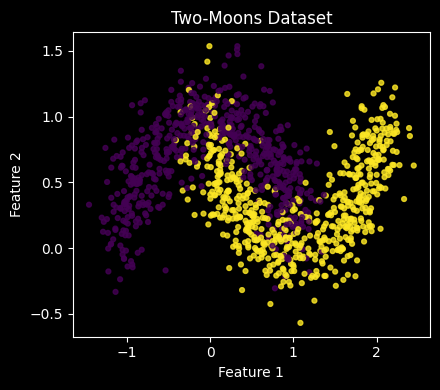
The experiments use a synthetic two-dimensional binary classification dataset commonly referred to as the two moons dataset. The dataset consists of two interleaving half-circle distributions and is frequently used to evaluate nonlinear decision boundaries in low-dimensional settings. While small, it is not linearly separable and therefore requires nonlinear transformations for accurate classification.
The dataset is generated procedurally using a fixed random seed to ensure reproducibility. A single train/validation split is applied and held constant across all experiments so that each initialization strategy is evaluated on identical data. This design isolates initialization effects from dataset variability.
The two-dimensional input space implies a small fan-in for the first dense layer. This amplifies the influence of weight initialization on early activations and gradients, making the dataset suitable for studying initialization dynamics directly.
Figure 1 visualizes the dataset with class coloring.
2.2 Model Architecture
All experiments use the same fully connected feedforward neural network. To better emulate real training behavior without making the experiment computationally heavy, the network includes multiple hidden layers and uses ReLU in the hidden stack. The output layer is softmax with categorical cross-entropy loss.
Architecture (fixed across runs):
2 → 64 → 64 → 64 → 2
The model is constructed using the build_model(weight_method) function shown in the introduction.

2.3 Weight Initialization Methods
Initialization is controlled inside Layer_Dense.__init__ in SaorsaNN_CPU.py. The study compares:
- Small normal (baseline):
0.01 * np.random.randn(...) - Glorot normal:
sd = sqrt(2/(fan_in + fan_out)), thenN(0, sd) - He normal:
sd = sqrt(2/fan_in), thenN(0, sd)
2.4 Controlled Randomness and Repeatability
Randomness is controlled at two levels:
- Dataset seed and split seed: Fixed to keep the task constant across all experiments.
- Model-level seeds: Varied across runs to measure run-to-run sensitivity caused by initialization randomness.
This design supports fair comparisons: each initialization strategy is evaluated on the same dataset and split, but across multiple independent initializations.
2.5 Training Configuration
All runs are:
- Optimizer: Adam
- Learning rate: 0.001
- Epochs: 250
- Batch size: None (one step per epoch for clarity and stable metric alignment)
- Regularization / dropout: not used
- Normalization layers: not used (see Discussion)
Metrics recorded per epoch include training loss and training accuracy, and final validation accuracy is computed from model.predict().
3. Results
This section presents empirical comparisons across initialization strategies.
3.1 Convergence Behavior
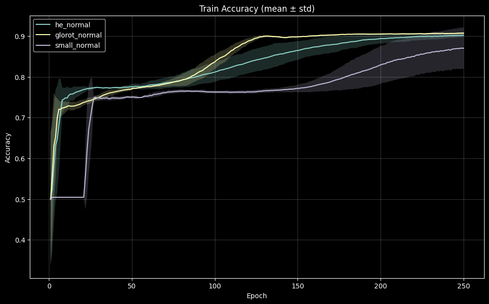
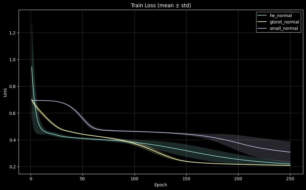
Figures 3 and 3b reveal clear differences in optimization dynamics induced by the initialization strategy. Glorot normal initialization exhibits both rapid early improvement in training accuracy and a smooth, steadily decreasing loss curve, accompanied by relatively tight variance bands across seeds. This behavior suggests that the initial weight scale produces gradient magnitudes that are well-aligned with the fixed Adam learning rate, resulting in stable effective step sizes during early training. In contrast, the small normal initialization (std = 0.01) shows slower early accuracy gains and wider inter-seed variability. The corresponding loss curves display greater oscillation and delayed stabilization, indicating that the initial weight distribution yields gradients that interact less predictably with the optimizer, leading to more variable update magnitudes across runs. He normal initialization converges reliably but exhibits moderately greater variance than Glorot under these conditions, particularly during the first several epochs. Although all three strategies ultimately approach similar accuracy plateaus, the transient training dynamics differ meaningfully, demonstrating that initialization primarily influences early gradient flow, effective update scaling, and optimization stability rather than ultimate representational capacity in this setting.
3.2 Variability Across Runs
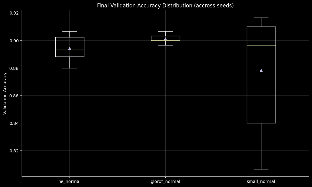
The distribution of final validation accuracy reveals clear differences in run-to-run stability across initialization strategies. Models initialized with Glorot normal exhibit the narrowest distribution, indicating consistent convergence outcomes across seeds. He normal shows moderately increased variability, while the small normal initialization (std = 0.01) displays the widest spread, with some runs converging noticeably less effectively than others.
These results indicate that, even when models ultimately reach comparable mean performance, initialization choice substantially influences the reliability and repeatability of training outcomes under fixed hyperparameters.
3.3 Learned Decision Boundaries
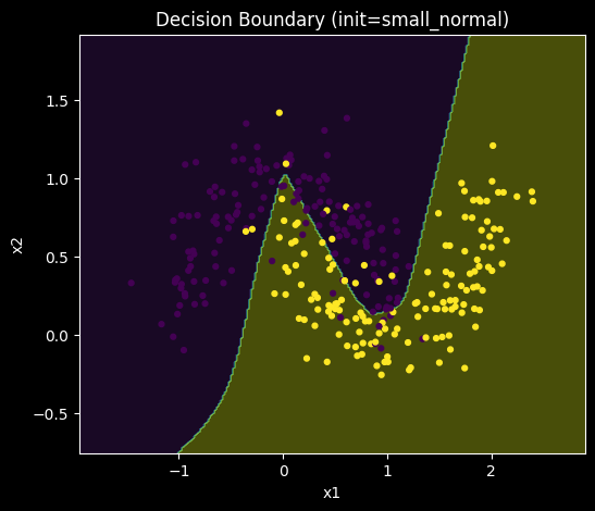
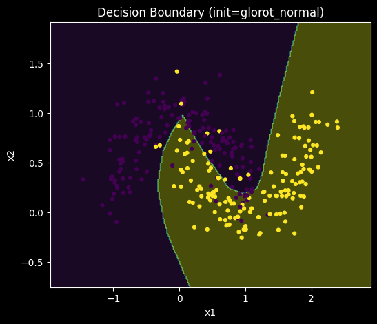
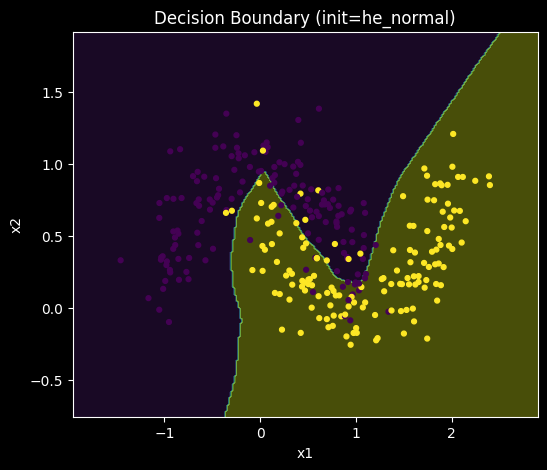
Figure 5. Decision boundaries learned by representative models trained under (a) small normal (std = 0.01), (b) Glorot normal, and (c) He normal initialization.
All three initialization strategies ultimately learn nonlinear decision boundaries capable of separating the two classes, indicating that model capacity is sufficient in all cases. However, qualitative differences are observable in boundary smoothness and symmetry. Models trained with Glorot normal initialization tend to produce more balanced and regular decision boundaries, while boundaries learned under small normal initialization appear more irregular and sensitive to local variations in the data.
These visual differences are consistent with the observed variability in convergence behavior and suggest that initialization affects not only training dynamics but also the geometry of the learned solution, even when final accuracy is similar.
3.4 Weight Evolution During Training
To complement scalar metrics, we also examine training dynamics at the parameter level by visualizing dense-layer weight matrices across epochs. Using the Visualize_Training utility, we recorded .mp4 animations of weight evolution for representative runs under each initialization strategy.
The Glorot and He initializations exhibit more gradual, subtle color transitions, consistent with smoother weight updates. In contrast, the small normal baseline shows more abrupt color shifts, indicating larger relative parameter changes and less stable weight evolution early in training.
Figure 6. Weight matrix evolution across training epochs for (a) small normal (std = 0.01), (b) Glorot normal, and (c) He normal initialization. Subtle color transitions indicate smoother parameter evolution; abrupt transitions indicate larger relative updates and less stable optimization dynamics.
4. Discussion
Although He initialization is theoretically well-matched to ReLU activations, it does not consistently outperform Glorot initialization in this experiment. One key factor is the low input dimensionality: the first dense layer has a fan-in of 2, which produces comparatively large initial weights under He normal relative to Glorot normal or a small normal baseline. Under a fixed Adam learning rate, this can increase early optimization sensitivity and widen run-to-run variability.
In contrast, Glorot normal produces a more conservative initial weight scale due to its dependence on both fan-in and fan-out. In this experimental regime, that smaller scale corresponds to smoother optimization trajectories, reduced variance bands, and more stable convergence behavior.
4.1 Interpretation and Practical Implications
These results suggest that initialization strategies should be selected with consideration for architectural and optimization context, not activation function alone:
- He (Kaiming) initialization is often advantageous for ReLU networks in deeper architectures or layers with moderate-to-large fan-in, where maintaining activation variance across many layers is critical.
- Glorot (Xavier) initialization can be favorable for shallow-to-moderate depth networks, early layers with very low-dimensional inputs, or when stability and repeatability across runs are prioritized.
- Small normal baselines can work on simple problems, but they may exhibit less stable optimization dynamics and greater run-to-run variability as model depth or task complexity increases.
More broadly, weight initialization is part of the optimization design space. It shapes early training dynamics and can reduce the need for extensive hyperparameter tuning when stability and reproducibility are important outcomes.
4.2 A Note on Normalization Layers
This study intentionally omits normalization layers (e.g., Batch Normalization or Layer Normalization) to isolate the effect of weight initialization. Normalization layers explicitly rescale activations during training and can mask behaviors that initialization strategies are designed to control. In normalized networks, differences between initialization strategies may appear less pronounced because normalization can stabilize activation magnitudes even when initialization is imperfect.
However, normalization does not eliminate the relevance of initialization. Early training dynamics before normalization statistics stabilize, optimizer interactions, and gradient magnitudes can still depend on initial weight scale. Moreover, normalization introduces additional parameters and constraints and may be undesirable in small models, inference-limited environments, or cases where batch statistics are unreliable. Initialization and normalization should therefore be viewed as complementary design decisions rather than interchangeable solutions.
5. Key Takeaways
- Weight initialization influences training stability and convergence speed under fixed training defaults.
- Low-dimensional inputs can amplify initialization effects in early layers.
- Under the conditions of this study, Glorot normal produced the most stable behavior across seeds.
- Weight-evolution visualizations provide an intuitive stability signal consistent with metric-based evaluation.
- Initialization remains a first-order training design choice, even when using adaptive optimizers.
6. Conclusion
This study demonstrates that weight initialization materially influences neural network training behavior, even in a controlled and relatively simple setting. Under a fixed architecture, optimizer, and learning rate, different initialization strategies produced measurable differences in convergence speed, run-to-run stability, and internal parameter dynamics. In this configuration, Glorot normal initialization yielded the most stable behavior across seeds, while small normal initialization exhibited greater variability during early training.
Although all strategies ultimately reached similar performance levels, the paths taken to reach those solutions differed meaningfully. These differences are not merely theoretical: initialization affects the number of epochs required to reach target performance, the consistency of outcomes across runs, and the smoothness of optimization trajectories. In practical terms, weight initialization therefore influences both training time and computational cost. Faster, more stable convergence reduces optimization steps, shortens experimentation cycles, and lowers resource expenditure. Even modest improvements in early training dynamics can translate into meaningful savings at scale. For these reasons, initialization should be treated as a deliberate design choice rather than an afterthought in model development.
References
- LeCun, Y., Bottou, L., Orr, G. B., & Müller, K.-R. Efficient Backprop. Neural Networks: Tricks of the Trade, 2012.
- Sutskever, I., Martens, J., Dahl, G., & Hinton, G. On the Importance of Initialization and Momentum in Deep Learning. ICML, 2013.
- Bengio, Y., Simard, P., & Frasconi, P. Learning Long-Term Dependencies with Gradient Descent Is Difficult. IEEE TNN, 1994.
- Glorot, X., & Bengio, Y. Understanding the Difficulty of Training Deep Feedforward Neural Networks. AISTATS, 2010.
- He, K., Zhang, X., Ren, S., & Sun, J. Delving Deep into Rectifiers: Surpassing Human-Level Performance on ImageNet Classification. ICCV, 2015.
- Goodfellow, I., Bengio, Y., & Courville, A. Deep Learning. MIT Press, 2016.


Leave a Reply